uLisp

Graphics examples

The following examples demonstrate the use of the graphics extensions, currently available in the RISC-V version of uLisp that supports the Sipeed MAiX range of RISC-V boards.

RGB utility

These routines make use of the following rgb utility to define a colour from its RGB components:

(defun rgb (r g b)
  (logior (ash (logand r #xf8) 8) (ash (logand g #xfc) 3) (ash b -3)))

Each of the parameters r, g, and b should be an integer from 0 to 255. For example, to define orange you could use:

(defvar *orange* (rgb 255 128 0))

Coloured ellipses

 

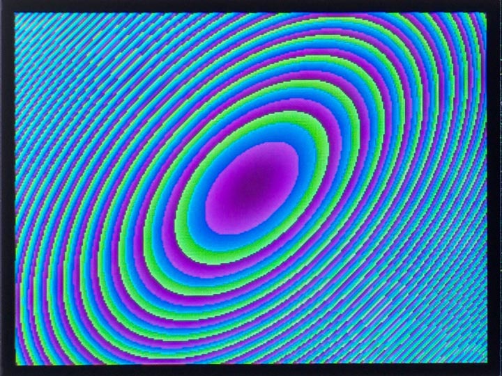
This simple demo displays a series of coloured ellipses:

(defun plot ()
  (dotimes (xx 320)
    (let ((x (- xx 160)))
      (dotimes (yy 240)
        (let* ((y (- yy 120))
               (f (truncate (+ (* x (+ x y)) (* y y)) 8)))
          (draw-pixel xx yy (rgb (+ f 160) f (+ f 80))))))))

It plots the value of x² + y² + xy as a function of x and y.

HSV utility

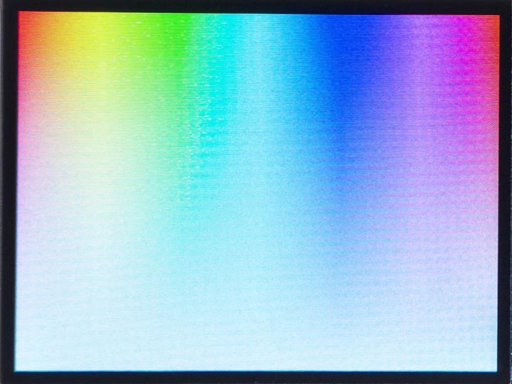
This routine allows you to specify colours in the alternative HSV colour system (also called HSB) ^[1].

(defun hsv (h s v)
  (let* ((chroma (* v s))
         (x (* chroma (- 1 (abs (- (mod (/ h 60) 2) 1)))))
         (m (- v chroma))
         (i (truncate h 60))
         (params (list chroma x 0 0 x chroma))
         (r (+ m (nth i params)))
         (g (+ m (nth (mod (+ i 4) 6) params)))
         (b (+ m (nth (mod (+ i 2) 6) params))))
    (rgb (round (* r 255)) (round (* g 255)) (round (* b 255)))))

It's useful because, for particular fixed values of s and v, you can generate a range of different colours of similar brightness and saturation simply by varying the h parameter.

It takes the following parameters:

• h is the hue, which can be from 0 to 359, representing degrees around a colour circle.
• s is the saturation, which can be from 0, representing white, to 1.0, representing 100% saturation.
• v is the value, which can be from 0, representing black, to 1.0, representing 100% brightness.

The following routine generates the plot shown above of hue horizontally against saturation vertically, with value = 100%:

(defun plot ()
  (set-rotation 2)
  (fill-screen)
  (dotimes (x 320)
    (dotimes (y 240)
      (draw-pixel x y (hsv (/ (* x 360) 320) (/ y 240) 1)))))

Mandelbrot set

This popular fractal function generates complex detail however far you zoom in to it ^[2].

For each point (x, y) the function repeatedly applies a transformation to the complex number represented by x + iy, and counts the number of iterations before the size of the value exceeds 2.

The number of iterations is plotted as a different colour, using the above hsv routine, or black if the function hasn't diverged after 80 iterations:

(defun mandelbrot (x0 y0 scale)
  (set-rotation 2)
  (fill-screen)
  (dotimes (y 240)
    (let ((b0 (+ (/ (- y 120) 120 scale) y0)))
      (dotimes (x 320)
        (let* ((a0 (+ (/ (- x 160) 120 scale) x0))
               (c 80) (a a0) (b b0) a2)
          (loop
           (setq a2 (+ (- (* a a) (* b b)) a0))
           (setq b (+ (* 2 a b) b0))
           (setq a a2)
           (decf c)
           (when (or (> (+ (* a a) (* b b)) 4) (zerop c)) (return)))
          (draw-pixel x y (if (plusp c) (hsv (* 359 (/ c 80)) 1 1) 0)))))))

The parameters x0 and y0 are the coordinates of the centre of the plot, and scale specifies the scale factor. To plot the whole Mandelbrot set call:

(mandelbrot -0.5 0 1)

The plot shown above zooms in on a detail, and was obtained with:

(mandelbrot -0.53 -0.61 11)

On a MAiX board at the default clock speed it took 127 s.

For a description of how to speed this up by writing the inner loop in RISC-V assembler see Mandelbrot set using assembler.

Sierpinski curve

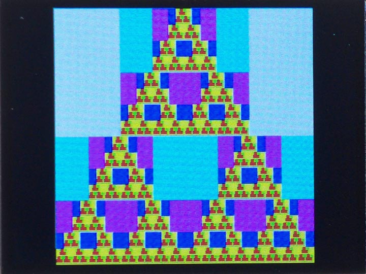
This is a recursively-defined curve. It starts with a triangle constructed from three squares; then each square is replaced by a triangle of smaller squares, and so on. Each generation is shown in a different colour:

(defun sierpinski (x0 y0 size gen)
  (when (plusp gen)
    (let ((s (ash size -1))
           (n (1- gen)))
      (fill-rect x0 y0 size size (col gen))
      (sierpinski (+ x0 (ash s -1)) y0 s n)
      (sierpinski x0 (+ y0 s) s n)
      (sierpinski (+ x0 s) (+ y0 s) s n))))

The following function col defines a different colour for each value of n from 0 to 7:

(defun col (n)
  (rgb (* (logand n 1) 160) (* (logand n 2) 80) (* (logand n 4) 40)))

Finally, this function draw draws the above plot showing 7 generations:

(defun draw ()
  (set-rotation 2)
  (fill-screen)
  (sierpinski 40 0 240 7)) 

---

1. ^ HSL and HSV on Wikipedia.
2. ^ Mandelbrot set on Wikipedia.